Image Arithmetic
As we discussed before, images are basically just matrices of pixel values that range from 0 to 255. And since they are built in this format, it is actually easy to perform arithmetic (math) on images, such as addition or subtraction.
There are many uses for performing image math. For the first example we will show what happens when we add two images together.
>>> imgA = Image("simplecv")
>>> added = imgA + imgA
>>> added.show()
So what we did was take the original simplecv image logo that looked like
and converted so it looked like this:

If you note that since ( X + X = X * 2) we can also try this as well.
>>> imgA = Image("simplecv")
>>> mult = imgA * 2
>>> mult.show()
You should get the same exact image as shown before. You can also perform subtraction. Except what is different here, is that using subtraction will only show what has changed between the two images.
>>> logo = Image("logo")
>>> sub = logo - logo
>>> sub.show()
You should get a completely black image.
..note: To perform image math the images have to be the same exact size
It is also possible to perform division on images. This is useful for lowering the contrast. For instance if you use the SimpleCV logo:
And if we divide the image by 10:
>>> scv = Image("simplecv")
>>> div = scv / 10
>>> div.show()
and you should get something that looks like:

Now you maybe asking when image math is actually useful. Well let’s give a quick example. We will show how simple subtraction can be used to detect motion. In this example we have a picture of a person, then the next picture you can tell they waved their hand. Then we will subtract those two images and you will only what has changed between the two images.
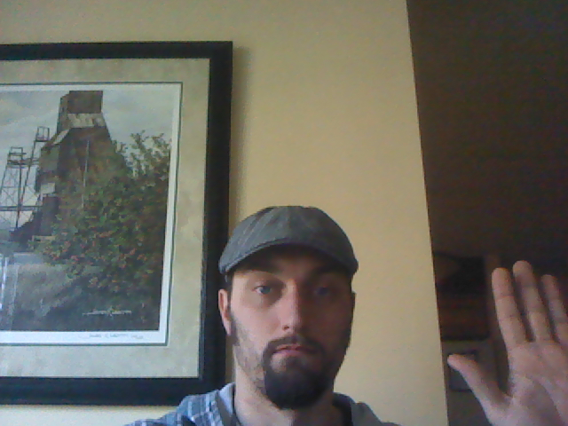
Previous Frame
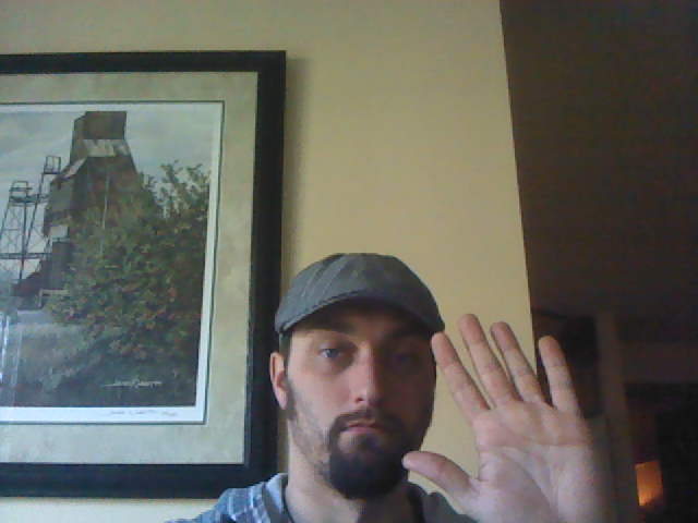
Current Frame
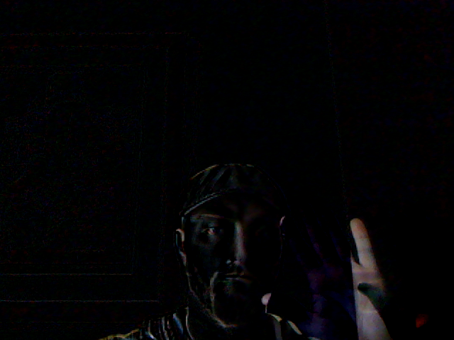
Difference Image
As seen above only the pixels that changed between the two images are shown. To perform a similiar example just do:
>>> cam = Camera()
>>> prev = cam.getImage()
>>> current = cam.getImage()
>>> diff = current - prev
>>> diff.show()
But how does that tell us that motion occured? Well we can use some basic math to figure that out. We know if the pixel value was black (0) then nothing had changed, but if not black, then something must have changed. We will compute how much of the entire picture actually changed.
To do this we will just get the image matrix and add a counter:
>>> area = diff.width * diff.height
307200 #this is our image area in pixels
>>> matrix = diff.getNumpy()
>>> matrix.shape
(640, 480, 3)
>>> flat = matrix.flatten()
>>> counter = 0
>>> for i in flat:
        if flat[i] == 0: #if black
                counter += 1

>>> percent_change = float(counter) / float(len(flat))
>>> print percent_change
0.818358289930555
With this you are able to determine about 0.8 or 80% change in pixels. Although this is not the most efficient way we can now use this change as a threshold value. For instance send an e-mail if 90% of the pixels change, and using a threshold you can minimize the chance of false positives happening.
As mentioned this probably isn’t the most effecient way to determine if motion has occured, but it is probably the most basic method and was just meant to show how you can use image math to do some basic useful things.
We can also use other properties of the image. For instance any standard type of mathematic statistics functions are available. This could be mean, standard deviation, etc. As in the previous example we could instead use the mean which is much quicker.
Let’s use that in a complete program below:
from SimpleCV import *

cam = Camera()
threshold = 5.0 # if mean exceeds this amount do something

while True:
        previous = cam.getImage() #grab a frame
        time.sleep(0.5) #wait for half a second
        current = cam.getImage() #grab another frame
        diff = current - previous
        matrix = diff.getNumpy()
        mean = matrix.mean()

        diff.show()

        if mean >= threshold:
                print "Motion Detected"
Exceptions in Image Math
In image math you will never have a negative number. This is because values will push the value. The values can be between 0 and 255, no more no less.
Examples:
200 - 255 = 0
100 + 200 = 255
0 + 300 = 255
If we remember, that color or greyscale still uses the 0 to 255 value. And keep in mind that white is all colors, and black is the absence of color. So if you were to add say a completely blue image to a white image the image would still be white, because:
white = (255,255,255)
blue = (0, 0, 255)
white + blue = (255, 255, 255)
And in fact you can verify this with the following code:
>>> black_img = Image((20, 20)) #make a 20 x 20 pixel black image
>>> black_img.show()
>>> blue_img = Image(black_img.getNumpy() + Color.BLUE)
>>> blue_img.show()
>>> white_img = black_img.invert()
>>> white_img.show()
>>> added_img = white_img + blue_img
>>> added_img.show()
Histograms
Another extremely useful tool when performing math on images is to use a histogram. A histogram is what is typically used in statistics, and is basically just a plot of the values in a list. These values can be anything really, from a list of the area of features found, to coordinates, etc. But what typically histograms are used for is a list of all the colors from each of the color channels in an image.
Earlier we talked about colors ranging from 0 to 255. And this is per channel on a grey image the same color is used across all channels. For instance let’s take a look at the histogram of the simplecv logo in grey.:
>>> img = Image('simplecv')
>>> gray = img.toGray()
>>> histogram = gray.histogram()
>>> len(histogram)
50
>>> print histogram
[1929,
 2562,
 ...
 0,
 2372]
This was a list of values as a frequency of their occurance in the image. In this case there are 50 values in this list. These are referred to as bins. You can change the number of bins by passing it as a value. For instance if we want to show all 255 values then just use.:
>>> histogram = gray.histogram(255)
>>> len(histogram)
255
Now we want to see what that actually looks like so we will plot it.
>>> plot(histogram)
and you should see an image similiar to.

Histogram of SimpleCV logo in Gray
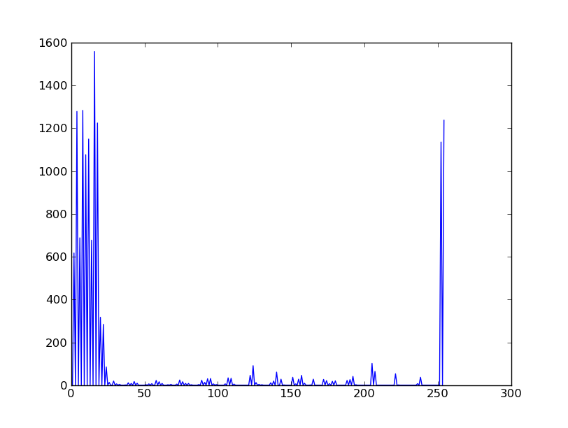
If you look at the above image you will see basically the distribution of the colors plotted. Since the image is gray, then you will notice a high frequency of occurances near the black (0) and white (255) end of the histogram, with not much in the middle. To verify this, let’s do the same plot with the color image to see the differences. But we also have to plot each color channel seperate, so Red, Green, and Blue all range from 0 to 255.
>>> img = Image('simplecv')
>>> (red, green, blue) = img.splitChannels(False)
>>> red_histogram = red.histogram(255)
>>> green_histogram = green.histogram(255)
>>> blue_histogram = blue.histogram(255)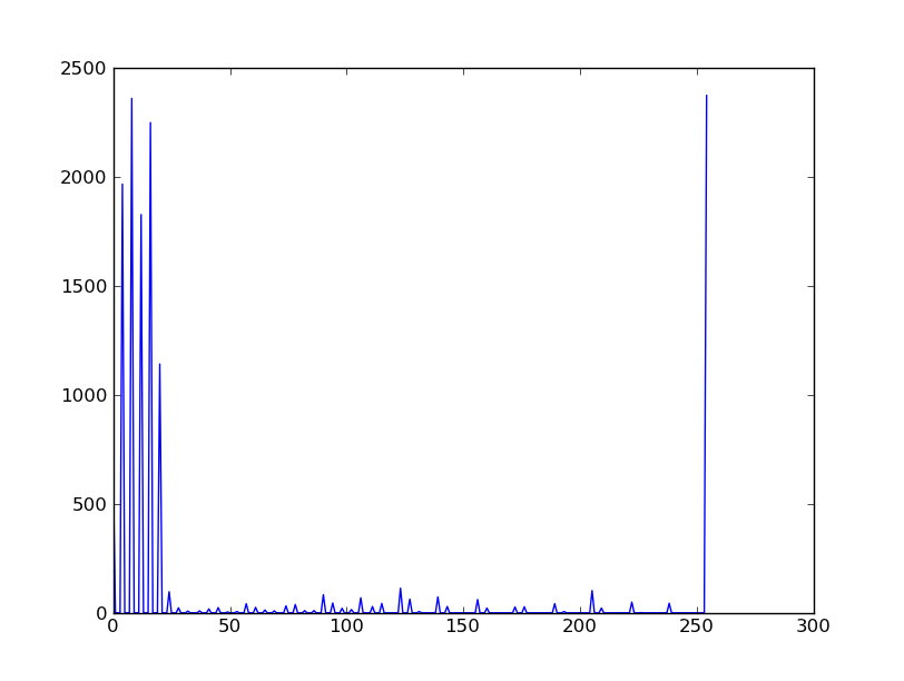
Histogram of SimpleCV logo Red Color Channel
Histogram of SimpleCV logo Green Color Channel
Histogram of SimpleCV logo Blue Color Channel
Color Space
Something that hasn’t been talked about too much is the idea of color space. Basically this is the method used to describe color. The most commonly used and well known color space is Red-Green-Blue (RGB). It’s similiar to something you may have seen in art class called the color wheel.
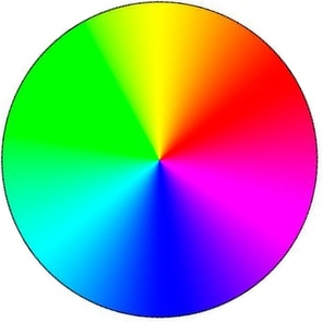
Image of Color Wheel
What color space is basically the way you figure out the color. For instance in RGB color space to get the color blue, it’s just (0,0,255) for the RGB values. There are many other ways to describe color. Another popular method is called Hue-Saturation-Value (HSV). This is another method to represent blue for instance, and it’s value in HSV is (240,100,100). Lets look at an example.:
>>> img = Image('simplecv')
>>> hsv = img.toHSV()
>>> histogram = hsv.histogram(255)
>>> print histogram
[34, 209, 408, 602, 676, 0, 688, 680, 603, 591, 485, 0, 546, 603, 677,
743, 0, 815, 689, 536, 317, 187, 0, 101, 56, 26, 12, 0, 10, 8, 5, 5, 4,
0, 0, 0, 2, 0, 0, 3, 4, 9, 10, 12, 0, 5, 4, 0, 0, 0, 0, 1, 3, 2, 0, 0,
7, 12, 10, 6, 0, 10, 10, 5, 2, 1, 0, 0, 1, 0, 0, 3, 0, 8, 13, 18, 16, 0,
4, 5, 1, 0, 2, 0, 9, 3, 3, 2, 0, 2, 21, 13, 15, 21, 0, 28, 3, 6, 2, 0,
0, 0, 0, 7, 6, 0, 11, 17, 15, 14, 0, 6, 2, 5, 27, 11, 0, 0, 0, 0, 0, 0,
18, 22, 38, 66, 15, 0, 1, 3, 1, 1, 0, 0, 18, 19, 1, 1, 0, 12, 26, 34, 14,
14, 0, 42, 2, 0, 0, 0, 0, 0, 0, 0, 11, 0, 59, 33, 13, 8, 0, 1, 0, 0, 0, 4,
0, 0, 0, 0, 0, 0, 4, 23, 21, 7, 0, 0, 0, 0, 0, 0, 0, 0, 0, 0, 0, 0, 0, 22,
20, 6, 0, 0, 0, 0, 0, 0, 0, 0, 0, 0, 0, 0, 26, 0, 76, 22, 0, 0, 0, 0, 0, 0,
0, 0, 0, 0, 0, 0, 0, 0, 33, 16, 1, 0, 0, 0, 0, 0, 0, 0, 0, 0, 0, 0, 0, 7,
0, 37, 0, 0, 0, 0, 0, 0, 0, 0, 0, 0, 0, 0, 0, 1135, 1237]
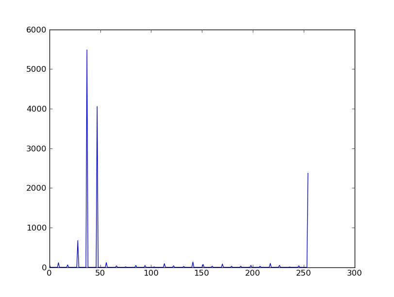
>>> plot(histogram)
As you can see the values are quite a bit different than the same image’s histogram using the RGB color space.
Histogram of SimpleCV logo using HSV colorspace
Now many of these different color spaces are used for many various things. In the case of HSV the first value, hue, can be adjusted to basically adjust the color level, so for instance if you wanted to shift the blue to a light blue then you can just adjust the hue channel. If you were using RGB color space, trying to adjust the “lightness” of the blue would require you to adjust 3 channel values.
For the most part you won’t have to muddle around with other color spaces. All the image algorithms can work the same in the color spaces, but color spaces make it easier to optimize for particular tasks. For instance maybe we wanted to check how blue something was. Using HSV we could easily use the saturation value as a threshold, so if it was above 80 but below 100. To do this using RGB would be much more complex.
please visit the wikipedia article if you would like to know more about colorspace: http://en.wikipedia.org/wiki/Color_space
Using Hue Peaks
The hue peaks function is used to help figure out what the dominant color in an image is. Using a histogram we can plot the values and see the actual peaks. What the huePeaks function does it make it convient to find this color. In this example we will use the lenna image to find the color (or hue) peaks.:
>>> lenna = Image('lenna')
>>> histogram = lenna.hueHistogram()
>>> print histogram
[13682 14520 12393 11312 10730 9966 9128 8128 7309 5738 4115 2624
1670 1252 1358 2110 2978 2430 1083 230 62 30 18 14
5 1 2 0 1 0 0 0 0 0 0 0
0 0 0 0 0 0 0 0 0 0 0 0
0 0 0 0 0 0 0 0 0 0 0 0
0 0 0 0 0 0 0 0 0 0 0 0
0 0 0 0 0 0 0 0 0 0 0 0
0 0 0 0 0 0 0 0 0 0 0 0
0 0 0 0 0 0 0 0 0 0 0 0
0 0 1 0 1 0 0 0 1 2 1 2
3 5 7 5 7 14 20 17 11 22 29 37
45 67 66 72 95 127 133 157 189 223 263 310
336 459 471 489 571 648 595 761 994 1087 1318 1590
1897 2357 3120 3674 4432 4480 4876 4798 4699 4292 3575 3055
2653 2510 2857 3287 4051 4720 5857 7496 9962 12562 26794]
>>> peaks = lenna.huePeaks()
>>> print peaks
[(162.0, 0.0186004638671875)]
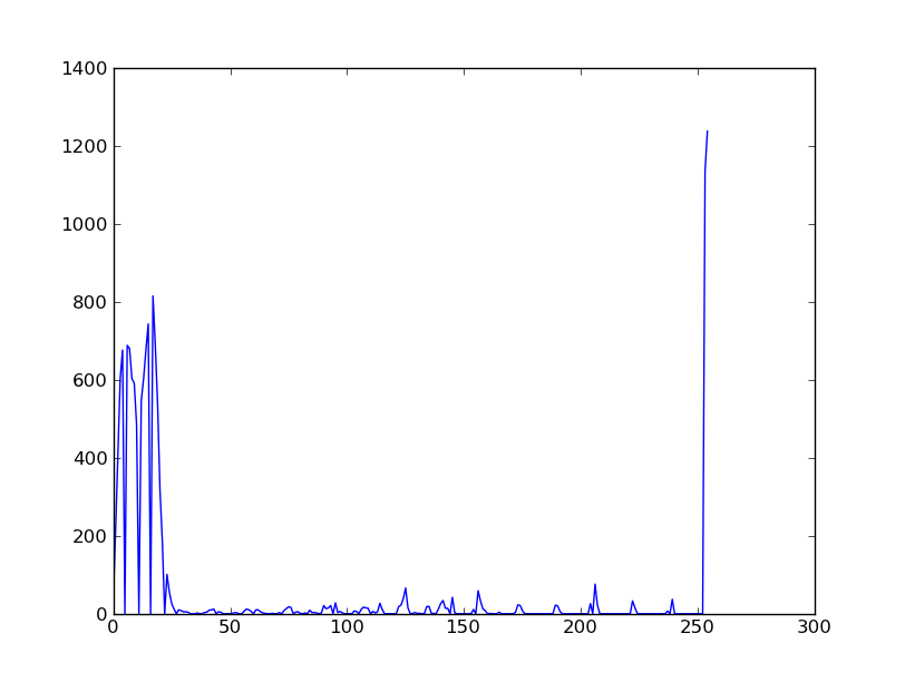
>>> plot(histogram)
Hue Histogram of Lenna Picture
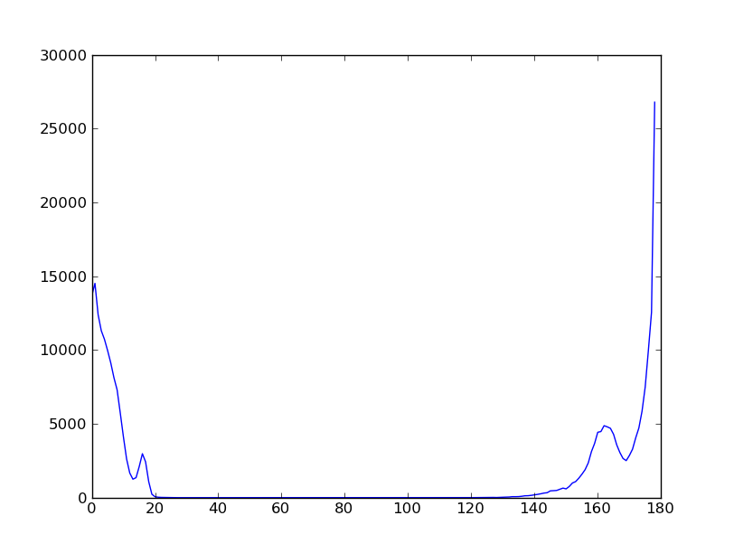
As you can see, the huePeaks() function list the value of 162, and looking at the plot you can see there is a peak there. Where this type of function maybe quite useful is trying to bring out the highest value color in the picture. To do this just use:
>>> lenna = Image('lenna')
>>> peaks = lenna.huePeaks()
>>> print peaks
[(162.0, 0.0186004638671875)]
>>> peak_one = peaks[0][0]
>>> print peak_one
162.0
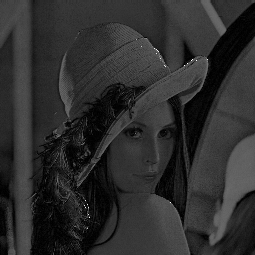
>>> hue = lenna.hueDistance(peak_one)
>>> hue.show()
Hue Distance of Lenna Image (blacker means closer to hue peak)
Creating a Motion Blur Effect
Here is a very good example of where you could use image math to add some effects to a video. Using some of the simple math functions built into python we can quickly do this to a live stream.
Let’s show the code:
from operator import add
from SimpleCV import *

cam = Camera()

frames_to_blur = 4
frames = ImageSet()

while True:
        frames.append(cam.getImage())

        if len(frames) > frames_to_blur:
                frames.pop(0)  #remove the earliest frame if we're at max

        pic = reduce(add, [i / float(len(frames)) for i in frames])
        #add the frames in the array, weighted by 1 / number of frames

        pic.show()
Let’s discus what is happening here. We load add from the operator library so we can ‘add’ the images back together. We set the frames_to_blur to 4, what this does is set the number of frames to basically blur together. We then create a ImageSet, this is basically a list of images with some built in options like mass saving the images in the list or viewing them. We then run through an infinite loop and keep adding images, if the number of frames added exceeds the number to blur then remove one from the list.
The reduce function is part of the standard python library. You may want to look some more into using map and reduce as functions in python as they are very quick and powerful. In this case we are using the add function to reduce all the images (or add them together). After they are summed into a single image they are then shown.
Simulating Long Exposure
Have you ever saw the type of art people can make using long exposure? Typically the images look something similiar to:
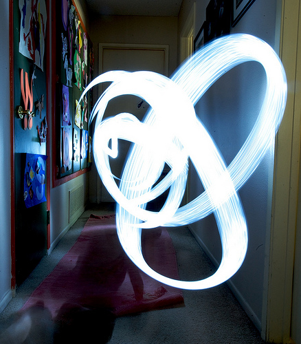
image taken from: http://www.flickr.com/photos/torres21/3688474968/
This is commonly refered to as light art. In this example we are going to simulate what is happening. Basically it’s just a sum of the images compressed into a single image.:
from SimpleCV import *

image_directory = "../static/images/exposure/"
frames = ImageSet() #create an empty image set
frames.load(image_directory) #load the directory of images
img = Image(frames[0].size()) #create an initial empty image
num_of_frames = len(frames) #count the number of images

for frame in frames:
        img = img + (frame / num_of_frames) # merge the images together

img.show()
time.sleep(1000)
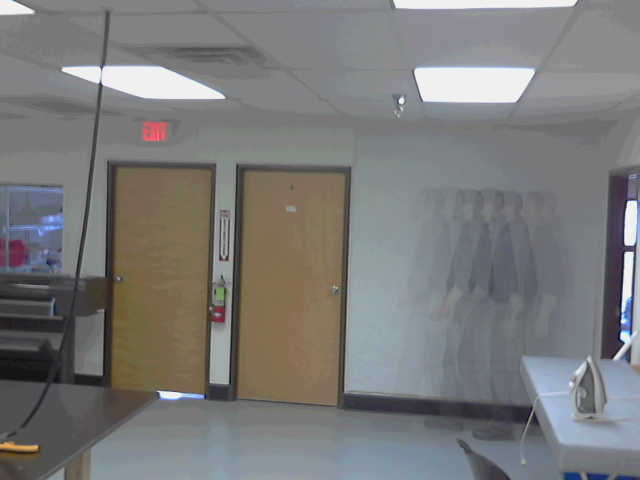
In our example we take a set of images, load them into memory, then run though that list and compress them. The images directory has about 10 images of a person walking by a wall. We create an imageset to store images in, this could be a list, but using the built in image set makes it much easier for us to load. We have to then create a empty image, this is used as a base to average the rest of the images against. We then run through the list of frames.
When ran we should get something that looks like:
Chroma Key (Green Screen)
We all have seen the weather reporter on television. They stand up in front of a screen and point to where storms maybe moving in, which direction the wind is moving, etc. The method they are doing this with is typically called a green screen. It is also (or used to be) one of the main methods to insert an actor into a movie or existing footage.
The way this is performed is basic image math, we are basically subtracting the certain colors we don’t want from that image. In our example we put our “anonymous” person in front of the green screen.
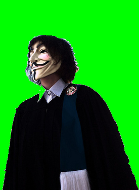
picture taken from: http://www.flickr.com/photos/pittaya/4785149065/
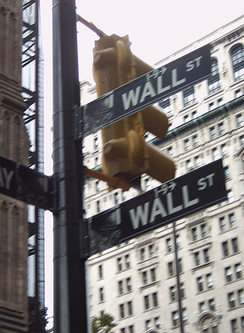
picture taken from: http://www.flickr.com/photos/willemvanbergen/271204700/
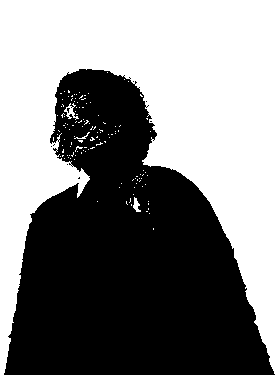
We use these pictures to create a mask. And no, pardon the pun, but not the mask the person is wearing in the picture. A mask has a similiar concept in image processing and in theory is similiar, you would wear a mask to hide your face, well a mask in image math is used to hide that part of the image. Our masked image should look something like:
To finally get something that looks like:
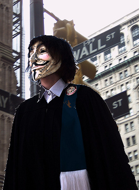
The code to perform a green screen is:
from SimpleCV import *

sleep_time = 2 #the amount of time to show each image for

#Load and show the greenscreen image
print "Showing Greenscreen image"
greenscreen = Image("../static/images/green-screen-person.png")
greenscreen.show()
time.sleep(sleep_time)


#load and show the background image
print "Showing background image"
background = Image("../static/images/green-screen-wallst.png")
background.show()
time.sleep(sleep_time)

#Create the mask to apply and show the mask
print "Showing Masked Image"
mask = greenscreen.hueDistance(color=Color.GREEN).binarize()
mask.show()
time.sleep(sleep_time)

#Combine the mask and other images to get the final result
print "Showing final image"
result = (greenscreen - mask) + (background - mask.invert())
result.show()
time.sleep(sleep_time)
Now performing the mask is similiar to what we did in the previous example using hue peaks. We used the hue distance to create the image and tell it to use green as the color, then we use binarize to either make it black or white as we need that for the image math.:
mask = greenscreen.hueDistance(color=Color.GREEN).binarize()
Now that we have the mask we do the actually image math with it:
result = (greenscreen - mask) + (background - mask.invert())
Here we are removing the mask from the green screen and adding it to the background with the inverted mask removed. You can think of it as cutting out a shape from one colored paper, and for it to fit into the big background piece of colored paper you would also have to remove that section from the background.